Model intercomparisons on terrestrial biogeochemistry

You can click here to download the 1st Version of the Protocol for model intercomparison on terrestrial carbon cycle with the traceability framework.

Brief introduction of a traceability framework for Model-intercomparison

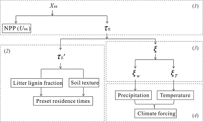
Biogeochemical models have been developed to account for more and more processes, making their complex structures difficult to be understood and evaluated. Based on the fundamental properties of terrestrial carbon cycle, we developed a framework which traces modeled ecosystem carbon storage capacity (Xss) to several traceable components. These components are (i) Xss as a product of net primary productivity (NPP) and ecosystem residence time (τE), (ii) baseline carbon residence times (τE’), (iii) environmental scalars (ξ), including temperature and water scalars, and (iv) environmental forcings. The relationships between the four components are organized as:

where NPP is net primary productivity, τE is ecosystem carbon residence time, τE' is baseline ecosystem carbon residence time, ξ is environmental scalar on carbon decay rates (ξw and ξT for water and temperature scalar, respectively).

This traceability framework has been successfully applied to the Australian Community Atmosphere Biosphere Land Exchange (CABLE) model to help understand differences in modeled carbon processes among biomes and as influenced by nitrogen processes. This framework is very useful for model intercomparisons on model structures of terrestrial biogeochemistry. More details about this study can be found in our paper on Global Change Biology (Xia et al. 2013).

Required output from the model

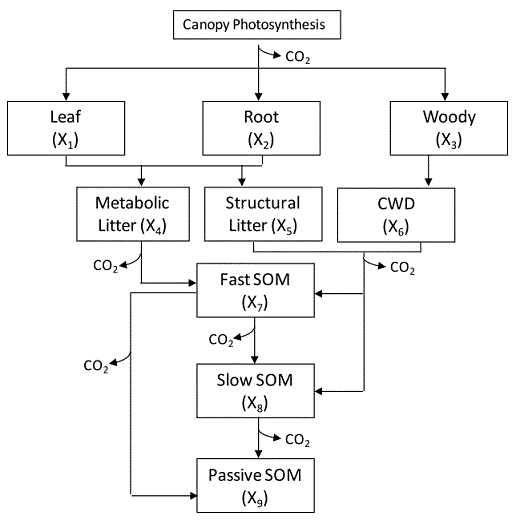
1. Develop a flow diagram to  represent model structure (box-arrow) as we have done for the CABLE model(this diagram is helpful but not required):

2. Find carbon balance equation for each of the pools with input and output (required);

3. Average NPP at steady state;

4. partitioning coefficient of NPP to each plant pool;

5. Potential mortality rate of each plant pool;

6. Adjusting factor for mortality rate (every scalars effect on mortality);

7. Transfer coefficient of dead plant tissue carbon from each plant pool to each litter pool;

8. Potential decay rate of litter from each litter pool;

9. Adjusting factor for potential decay rate;

10. Carbon transfer from each litter pool to each of soil pool;

11. Potential decomposition rate of soil organic carbon from each of soil pool;

12. Adjusting factors for decomposition rate;

13. Carbon transfer from each of soil pool to other soil pools.

 

Required variables

In order to make the required outputs more clear, we summarized them into the following table:

Variable	Associated Component	Deblahion
Net primary production (NPP)	Carbon influx
Allocation of NPP to leaf biomass	B vector	dimensionless;
Allocation of NPP to root biomass	B vector	dimensionless;
Allocation of NPP to woody biomass	B vector	dimensionless;
Transfer coefficient from leaf biomass to metabolic litter	A matrix	dimensionless;
Transfer coefficient from leaf biomass to structural litter	A matrix	dimensionless;
Transfer coefficient from woody biomass to CWD	A matrix	dimensionless; As '1' since all woody biomass transfer to CWD.
Transfer coefficient from metabolic litter to fast SOM	A matrix	dimensionless;
Transfer coefficient from structural litter to fast SOM	A matrix	dimensionless;
Transfer coefficient from structural litter to slow SOM	A matrix	dimensionless;
Transfer coefficient from CWD to fast SOM	A matrix	dimensionless;
Transfer coefficient from CWD to slow SOM	A matrix	dimensionless;
Transfer coefficient from fast SOM to slow SOM	A matrix	dimensionless;
Transfer coefficient from fast SOM to passive SOM	A matrix	dimensionless;
Transfer coefficient from slow SOM to passive SOM	A matrix	dimensionless;
Potential turnover rate of leaf biomass	C matrix	year-1;
Potential turnover rate of root biomass	C matrix	year-1;
Potential turnover rate of woody biomass	C matrix	year-1;
Potential turnover rate of metabolic litter	C matrix	year-1;
Potential turnover rate of structural litter	C matrix	year-1;
Potential turnover rate of CWD	C matrix	year-1;
Potential turnover rate of fast SOM	C matrix	year-1;
Potential turnover rate of slow SOM	C matrix	year-1;
Potential turnover rate of passive SOM	C matrix	year-1;
Water limitation on leaf biomass	Water scalar (ξw)	dimensionless;
Water limitation on root biomass	Water scalar (ξw)	dimensionless; as '1' in the CABLE model
Water limitation on woody biomass	Water scalar (ξw)	dimensionless; as '1' in the CABLE model
Water limitation on decomposition of metabolic litter	Water scalar (ξw)	dimensionless;
Water limitation on decomposition of structural litter	Water scalar (ξw)	dimensionless;
Water limitation on decomposition of fast SOM	Water scalar (ξw)	dimensionless;
Water limitation on decomposition of slow SOM	Water scalar (ξw)	dimensionless;
Water limitation on decomposition of passive SOM	Water scalar (ξw)	dimensionless;
Temperature limitation on leaf biomass	Tempearture scalar (ξT)	dimensionless;
Temperature limitation on root biomass	Tempearture scalar (ξT)	dimensionless; as '1' in the CABLE model
Temperature limitation on woody biomass	Tempearture scalar (ξT)	dimensionless; as '1' in the CABLE model
Temperature limitation on decomposition of metabolic litter	Tempearture scalar (ξT)	dimensionless;
Temperature limitation on decomposition of structural litter	Tempearture scalar (ξT)	dimensionless;
Temperature limitation on decomposition of fast SOM	Tempearture scalar (ξT)	dimensionless;
Temperature limitation on decomposition of slow SOM	Tempearture scalar (ξT)	dimensionless;
Temperature limitation on decomposition of passive SOM	Tempearture scalar (ξT)	dimensionless;
Pool size of leaf	Steady-state pool size (Xss)	g C m-2;
Pool size of root	Steady-state pool size (Xss)	g C m-2;
Pool size of woody biomass	Steady-state pool size (Xss)	g C m-2;
Pool size of metabolic litter	Steady-state pool size (Xss)	g C m-2;
Pool size of structural litter	Steady-state pool size (Xss)	g C m-2;
Pool size of CWD	Steady-state pool size (Xss)	g C m-2;
Pool size of fast SOM	Steady-state pool size (Xss)	g C m-2;
Pool size of slow SOM	Steady-state pool size (Xss)	g C m-2;
Pool size of passive SOM	Steady-state pool size (Xss)	g C m-2;
Annual total precipitation	Forcing	mm
Annual air temperature	Forcing	K

Desired model information

1. Response functions of carbon process to temperature and precipitation (or moisture ), or individual response functions for each pool);

2. Soil texture map;

3. Response functions to link soil texture to soil C processes;

4. Lignin fraction and other associated factors in affecting litter C processes;

5. Vegetation map.

Common guidelines for model runs

Each model can use their own forcings to drive the model, and specific spin-up method to run the model to steady state. Here are some common requirements for the model outputs:

(1) Models outputs should be obtained from the steady state;

(2) No additional simulations are needed for this model intercomparion, but the modelers should find the variables in Table 1 in their models and output them at the end of spin-up simulation.

(3) All the variables in the Table 1 are required as temporal averages from the steady-state run, but daily outputs of all variables are preferred.

Distribution policy

The traceability framework is distributed free to the academic community on the following conditions:

*Works based on the traceability framework leading to scientific publications should cite the paper published by Xia et al. (2013).

Reference

Xia JY, YQ Luo, YP Wang, O Hararuk. Traceable components of terrestrial carbon storage capacity in biogeochemical models. Global Change Biology 19(7)：2104–2116.[Download PDF]